In this post, I show you how to look up data based on criteria in multiple columns using XLOOKUP.
XLOOKUP is a more powerful, versatile, and user-friendly Excel lookup function that replaces the older VLOOKUP, allowing you to search left or right, return multiple columns, and handle errors gracefully with its default exact match and optional “if not found” value. VLOOKUP is limited to searching only to the right of the lookup column and requires a static column index number, making it more prone to errors when the table structure changes.
For this example, I’m working with a spreadsheet of Portlandia TV series data and I want to add the title of the episode to the list of characters based on season and episode numbers which are stored on another sheet in my workbook. To do this, I have to tell Excel to combine the season and episode numbers, then use the XLOOKUP function to pull the corresponding episode title based upon season and episode numbers.

NOTE: XLOOKUP only works in Excel 365 or 2021+. If you do not have XLOOKUP, I recommend creating a “helper column” where data can be concatenated (e.g., season-episode), then using VLOOKUP. Replacing XLOOKUP with VLOOKUP will not work in the example shown below.
Breaking Down the Formula
When using XLOOKUP for this example, we’ll need to do 3 things:
- Create a unique lookup value by combining the season and episode numbers separated by a hyphen
- Define the lookup array in the source data sheet, combining season and episode numbers using the same method
- Tell Excel where to look to find the result, which is the episode name in this example
Formula: =XLOOKUP(A2 & “-” & B2, ‘Episodes List’!A:A & “-” & ‘Episodes List’!B:B, ‘Episodes List’!C:C)
Where:
- A2 & “-” & B2 – creates the lookup value of season-episode (1-1)
- ‘Episodes List’!A:A & “-” & ‘Episodes List’!B:B – defines the lookup array, combining the season and episode numbers
- ‘Episodes List’!C:C – defines the return array (tells Excel to pull the match from the episode title column)
Step-by-Step Instructions
The following steps demonstrate how to use XLOOKUP in Excel for multi-criteria searches.
Insert a New Column for the Data
Insert a new column where the lookup data will be returned, if necessary. This can be done by selecting the column where the data will go and pressing ctrl and + or right click on the column and choose “insert.” I then typed “Title” into the top cell, C1, since that’s the data I’m adding and I expanded the width of the column.

Insert the XLOOKUP Function
Next, click in the cell in which you want the return data to appear. In my example, this is cell C2 where I will want the episode name to appear. We will copy the formula down the rest of the column later, so just start in the first cell.
Then click on the “insert function” button as shown below, locate and select the XLOOKUP function, then click OK.

This will open the function arguments modal in which we’ll enter the criteria for XLOOKUP.
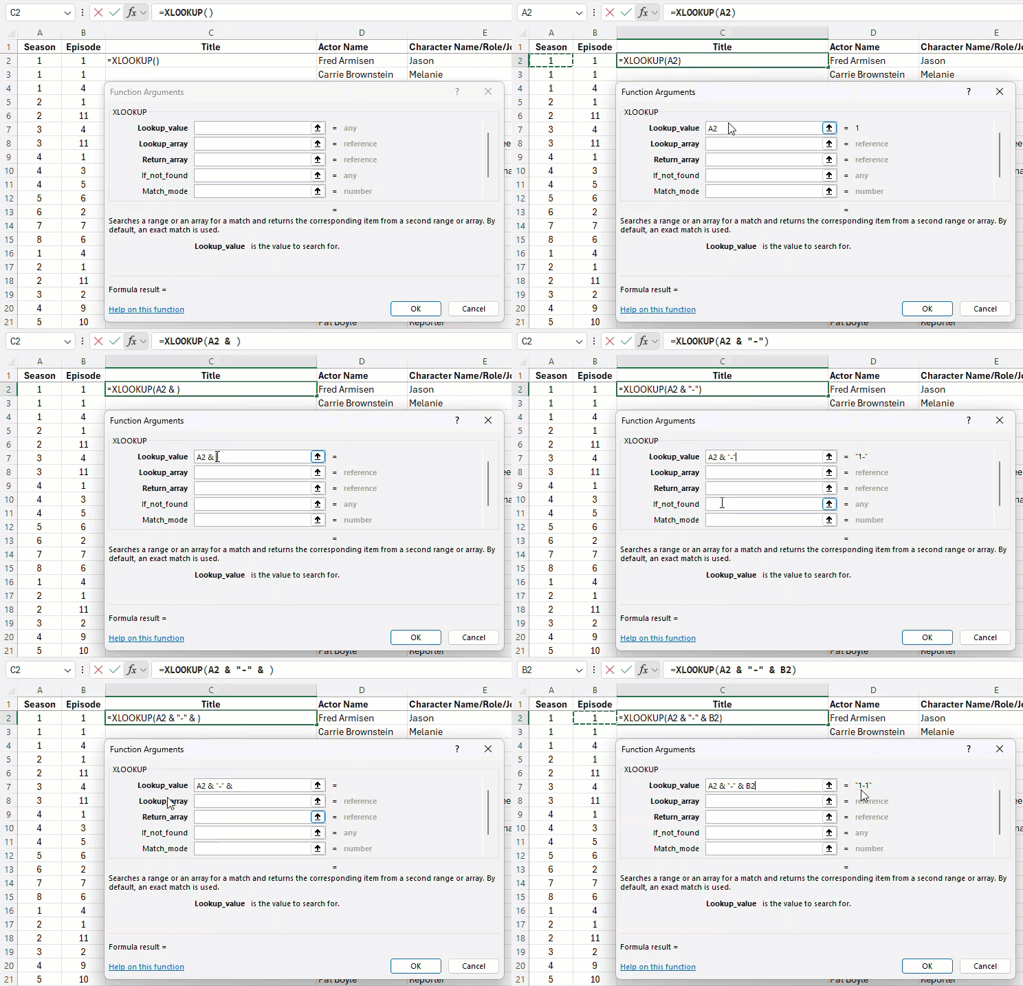
Create the Lookup Value
Since I need to combine the data in column A and B, I’ll do that using the & symbol with a hyphen in between:
- click in the lookup value field
- click in cell A2 to select the first value (season number)
- type & “-” & then clicking in cell B2 to tell Excel to join the episode number to the season number, separated by a hypen
- check the result to ensure “1-1” is displayed as the expected result
- What I typed: A2 & “-” & B2
Note: Use whatever connector you prefer and add spaces if desired, just be sure to enclose it in quotation marks so Excel knows this is to be used as a text value and use the same exact connector for the lookup array. If you have additional data to combine, repeat the steps to add the cells as needed.

Define the Lookup Array
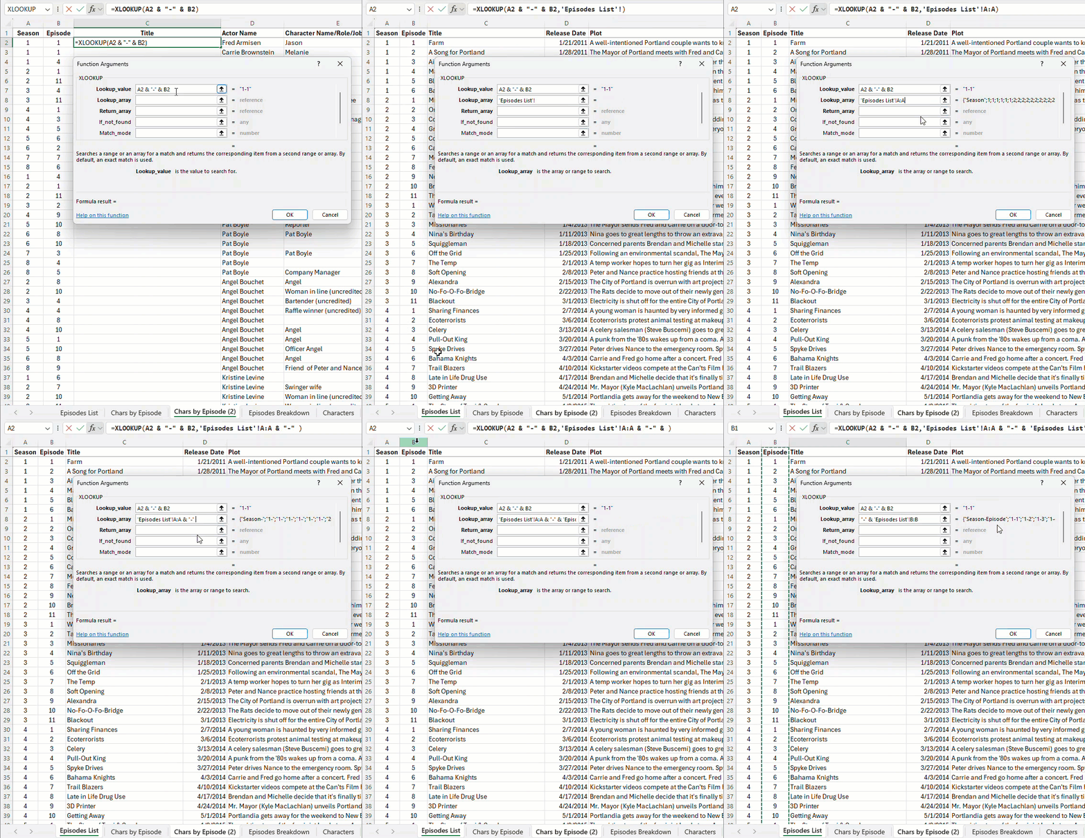
Next we’ll enter the lookup array. This tells Excel where to look for matching data and since the array also includes 2 columns of data, we’ll have Excel join it as we did in the previous step. It’s important to use the same exact connector for both the lookup and array values so Excel can properly match the values to produce the correct return value.
- Click in the lookup array field
- Click on the tab of the sheet containing the source data
- Click above the first column that contains the data to select the column
- Type & “-” & then click above the second data column to select the column – this will join the season and episode together, separated by a hyphen, exactly as done for the lookup value
- Check the result to ensure the source data tab is listed and the values are displaying as expected (e.g. “Season-Episode” ; “1-1” ; “1-2”)
- What I typed: ‘Episodes List’!A:A & “-” & ‘Episodes List’!B:B

Define the Return Array
Next, we need to tell Excel where to look for the return value, which is the episode title in this example.
- Click in the return array field
- Click on the tab of the sheet containing the return data
- Click above the column that contains the return data to select the column
- Check the formula result to ensure the source data tab is listed and the result shown below the argument fields is the correct answer (in this example, for season 1 episode 1, the correct answer is Farm)
- If everything looks correct, click OK to accept the formula
- What I typed: ‘Episodes List’!C:C

Copy the Formula Down the Column
Lastly, we’ll want to copy this formula down the rest of the column to provide the episode title for every row. I’ll show 2 methods below.
Note: If you are working with a lot of data, it can take several seconds for the data to populate and Excel may freeze briefly while doing this and it’s possible Excel could crash, so it’s a good idea to save your workbook before proceeding.
The Double Click Method
- Click the cell with the formula to select it
- Hover over the bottom right corner so the cursor changes to a thin black +
- Double click on the bottom right corner and the cells will auto-populate with data

The Drag Method
- Click the cell with the formula to select it
- Hover over the bottom right corner so the cursor changes to a thin black +
- Click once and hold, dragging the formula down the column

Don’t forget to subscribe to my YouTube channel for more tutorials!
Watch Portlandia on Amazon Prime Video
Note: As an Amazon Associate I earn from qualifying purchases.

