
Standard drop-down lists work well for short lists, but they quickly become difficult to use when you’re working with dozens or hundreds of options. A searchable drop-down list makes it much easier for users to find exactly what they need without scrolling through long lists.
In this tutorial, you’ll learn how to create a searchable drop-down list in Microsoft Excel by combining the FILTER function, named ranges, and Data Validation. You’ll also learn how to return partial matches, require exact matches, or perform case-sensitive searches depending on your needs. The included practice workbook contains examples for all three approaches so you can adapt them to your own spreadsheets
What You’ll Learn
- Create a searchable drop-down list in Microsoft Excel.
- Filter a list of options as you type.
- Return partial matches using the
SEARCHfunction. - Require exact or case-sensitive matches using
FILTERandEXACT. - Create a dynamic named range for Data Validation.
- Adapt the technique for customer lists, inventory, products, and other datasets.
Follow Along
Follow along using the interactive workbook created for this tutorial. It includes sample data, detailed formula explanations, and three separate worksheets demonstrating:
- Partial Matches
- Exact Matches
- Case-Sensitive Matches
The workbook also includes formula versions for both Microsoft 365 and older versions of Excel, making it easy to follow along regardless of which version you’re using.
The workbook is view-only in Google Sheets. You can create your own copy or download it as a Microsoft Excel workbook to experiment with the formulas using your own data.
Common Uses
Searchable drop-down lists are useful anytime users need to choose from a large list of values. Common examples include:
- Customer or contact lists
- Product catalogs
- Inventory management
- Employee directories
- Vendor lists
- Part numbers or SKUs
- Project or job tracking
- Event registration forms
Requirements & Compatibility
Requirements
This tutorial uses:
- The FILTER function
- SEARCH
- EXACT
- Named Ranges
- Data Validation
Compatibility
The primary method demonstrated uses the FILTER function, which is available in Microsoft 365 and Excel 2021 or later.
If you’re using Excel 2019 or earlier, the companion workbook includes an alternative approach, and you may also want to consider using an ActiveX Combo Box to create a similar searchable experience.
Comparison Table
The search types used in this tutorial:
| Search Type | Finds | Best Used When |
|---|---|---|
| Partial Match | Any item containing the search text | Users may only know part of a name or product. |
| Exact Match | Only identical values | Users must select a specific value. |
| Case-Sensitive Match | Identical values with matching capitalization | Codes, IDs, or situations where case matters. |
Step-by-Step Instructions
Below I outline the steps needed to create a searchable drop-down list in Excel.
Create a List of Options
The first step is to create a list of items you would like to be available in the drop-down list. These will be referred to as “options” in the following steps.
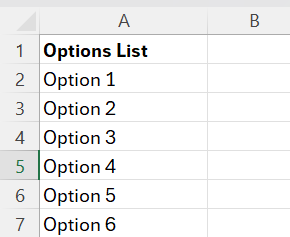
I entered the options in column A with a column header “options list” in cell A1 and all options listed below from A2 down.
This list is what will be filtered when entering a search term in the search box we’ll add next.
Choose a Cell for the Search Box & Drop-down list
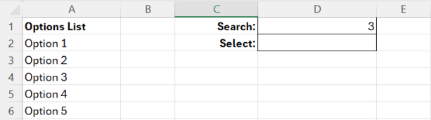
Next we want to decide where the search box should be located. This is the cell where the searching will be performed. I find it helpful to add a border around the cell and enter “search:” in the cell to the left so it’s easy to know where search terms can be entered.
I also chose a cell for the drop-down list that we will create in the last step of this process. I simply added a border around cell D2 and entered “select:” in the cell to the left like I did for the search box.
Use the FILTER Function to Generate Search Results
In this step, we will use the FILTER function to generate search results based upon what is entered in the search box we created in the previous step. This step will filter your list of options from step 1 based on what is entered in the search box from step 2.
I’m including 3 different FILTER choices so you can choose whether to allow partial matches, require exact matches, or require exact case-sensitive matches. In my video, I chose to allow partial matches so I don’t need to enter the full option name nor use the same upper/lower case as the option.
| Match Type | Results | Formula |
|---|---|---|
| Partial | Entering 3 will display any results containing 3, e.g., 3, 13, 403 | =FILTER(A2:A200, ISNUMBER(SEARCH(D1, A2:A200)), “”) |
| Exact | The search term must exactly match the option but is not case sensitive. e.g., entering “will” would NOT include “William” as a result; would need to search for “william” or “William” | =FILTER(A2:A200, A2:A200=D1, “”) |
| Case-sensitive exact | This search term must exactly match the option and is case-sensitive. e.g., entering “andrew” will NOT include “Andrew” as a result; would need to search for “Andrew” | =FILTER(A2:A200, EXACT(A2:A200, D1), “”) |
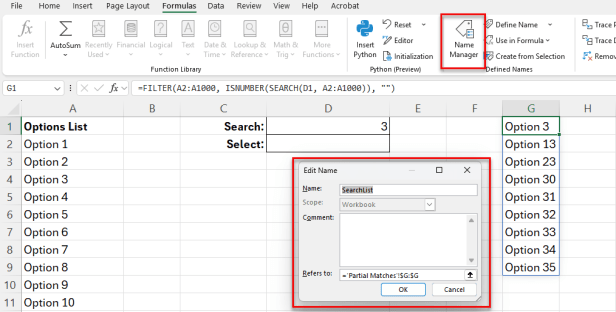
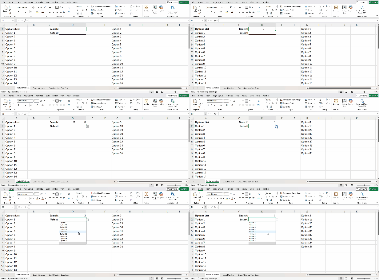
In my video, I chose to filter the results in column G, so I entered the partial match formula in cell G1. By default, all options will be displayed in column G, but once a value is entered in the search box (D1), the results will be filtered to display only results that match the value entered in the search box based on the type of matching selected.

Create a Named Range for the Filtered Results List
Next we will create a named range for the filtered results list we created in the last step. This is how we will tell the drop-down list where to find the filtered results in the next step.
- To create the named range, click on the Formulas tab then Name Manager
- Click “new” to create a new named range
- The name should be something easy to remember and type since we will be entering this name in the next step. I named mine “SearchList”
- In the refers to section, click on the arrow and select the column where your search results are. In my example, the results are in column G so I clicked on the G column header to select the entire column. The results may also included the sheet name.
- Click OK then close the name manager once done.
Apply Data Validation to Create the Drop-down List
The final step is to create the drop-down list using the data validation tool.
- Click in the cell where you want the drop-down box to be. Earlier, I chose cell D2 for this.
- Click on the Data tab, then click on the Data Validation button in the data tools section.
- On the settings tab, in the “allow” section, choose “list”
- In the source section, we’ll want to enter the name range we created in the last step preceded by the equals sign, so in my example I type =SearchList
- Click OK (if you receive an error, it likely means the source name was entered incorrectly, so double check that to ensure it is entered properly)

And that’s it! You should now be able to enter a value in your search box which filters the results that will be available in the drop-down list.
Additional Tips
Helpful Tip
If your list contains duplicate values, consider removing duplicates before creating the searchable drop-down. This provides cleaner search results and makes the list easier to navigate.
Version Differences
Microsoft 365 users can take advantage of dynamic array formulas such as FILTER, while older versions of Excel require alternative formulas or form controls. Both approaches are included in the downloadable workbook.
Related

How to Remove Extra Spaces in Excel
Learn how to remove extra spaces from text in Microsoft Excel using the TRIM function. This beginner-friendly tutorial explains what TRIM removes, when to use it, and why it’s one of the most useful functions for cleaning imported or inconsistent data.


How to Create an Order Form with Drop-Down Menus in Microsoft Excel
Learn how to create a professional order form in Microsoft Excel using drop-down menus, Data Validation, and named ranges. This step-by-step tutorial also covers formatting dates, ZIP codes, and credit card fields to build cleaner, more accurate spreadsheets for real-world business use.
Stay Updated
There are two easy ways to get notified when new tutorials are published:
Subscribe on YouTube for new video tutorials: @SimpleSoftwareTutorials
or enter your email below to receive new blog posts directly in your inbox:

