

Manually entering customer information over and over can be time-consuming and increase the risk of errors. By combining a drop-down list with the VLOOKUP function, you can automatically populate related information such as customer names, addresses, phone numbers, or other details with a single selection.
In this tutorial, you’ll learn how to create a drop-down list using Data Validation and use VLOOKUP to automatically fill multiple fields based on your selection. This walkthrough demonstrates a practical business example and can easily be adapted for order forms, packing lists, customer databases, contact lists, and many other Excel projects.
What You’ll Learn
In this tutorial, you’ll learn how to:
- Create a drop-down list using Excel’s Data Validation feature.
- Use the VLOOKUP function to retrieve related information automatically.
- Use the IFERROR function to display a blank cell instead of an error message.
- Auto-populate multiple fields from a single selection.
- Reduce repetitive data entry and improve accuracy.
- Apply the technique to real-world spreadsheets such as order forms, packing lists, customer databases, and contact management systems.
Practice & Resources
Updated Companion Guide
This tutorial is based on a video originally published in 2017. While the video still demonstrates the core technique, the written guide and downloadable resources have been updated where appropriate to reflect current Excel features, best practices, and version compatibility.
Click the button below to view the updated practice spreadsheet for this tutorial.
Video Tutorial
Note: This tutorial is based on a video originally published several years ago. The formulas shown in the downloadable workbook and written guide have been updated to reflect current Excel best practices. In particular, I’ve wrapped the VLOOKUP formula in IFERROR to prevent error messages from displaying when no selection has been made. This small improvement makes the worksheet more user-friendly while preserving the same overall approach demonstrated in the video.
Common Uses
- Customer order forms
- Packing lists
- Sales quotes
- Contact directories
- Inventory lookups
- Employee records
Breaking Down the Formula
The formula used in this tutorial:
=IFERROR(VLOOKUP($B$3,Customers!$A:$I,2,FALSE()),””)
Here’s that formula broken into its pieces:
=IFERROR( ... , "") This is the outer wrapper. It says: “try to run the formula inside, and if it produces an error, just show a blank cell instead of an ugly error message like #N/A.” That’s why when B3 is empty, the field shows nothing instead of an error.
VLOOKUP($B$3, Customers!$A:$I, 2, FALSE()) This is the actual lookup, and it has four parts:
$B$3– the thing you’re searching for. In this case, it’s the account number typed (or picked from the dropdown) in cell B3. The dollar signs lock that reference in place, so if you copy this formula to other cells, it still always looks at B3 and doesn’t shift to B4, B5, etc.Customers!$A:$I– where to search. This tells Excel to look at the entire A through I columns on the “Customers” sheet. VLOOKUP always searches the first column of this range (column A, which holds the account numbers) to find a match.2– which column to pull the answer from, counting from the left edge of the range you gave it. Column A is “1,” column B is “2,” and so on. Since column B on the Customers sheet holds Customer Name, a “2” here means “give me the name.”FALSE()– this means “only give me an exact match.” If it’s set to TRUE (or left out), Excel might return an approximate match instead, which isn’t what you want here; you need the exact customer tied to that exact account number.
Put together: “Take whatever account number is in B3, find that exact number in the Customers sheet, and bring back the value from the 2nd column of that row (Customer Name). If anything goes wrong – like B3 being blank – just show nothing instead of an error.”
The other fields on your Order Form (Attention, Address 1, City, etc.) use this exact same formula, just with the column number changed to 3, 4, 5, and so on, since each of those pieces of information lives in a different column on the Customers sheet.
Step-by-Step Instructions
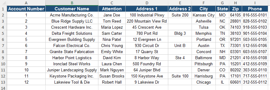
Step 1: Prepare Your Customer Data (Sheet2)
- Create a sheet that contains all customer information.
- Organize it in columns such as:
- Account Number | Customer Name | Attention | Address 1 | Address 2 | City | State | ZIP | Phone
- Make sure the column order matches the order you want to populate on your form.
Step 2: Create a Named Range for the Account Numbers
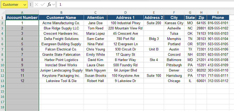
- Highlight the entire Account Number column — start at the first customer and drag down far enough to cover future customers (e.g., down to row 1000).
- Click the Name Box (top-left, next to the formula bar).
- Type a name for the range, e.g., Customer.
- Press Enter to save the named range.
Step 3: Create the Dropdown List (Sheet1)
- Go to your order form sheet.
- Click the cell where the dropdown should appear.
- Go to Data → Data Validation.
- Under Allow, choose List.
- In Source, type: =Customer
- (This references the named range you created.)
- Click OK — your dropdown is now ready.

Step 4: Insert the First VLOOKUP Formula
You’ll now make each field auto‑populate based on the dropdown selection.
- Click the cell where the Customer Name should appear.
- Insert a VLOOKUP formula: =IFERROR(VLOOKUP($B$3,Customers!$A:$I,2,FALSE()),””)
- Explanation of this formula is in the Breaking Down the Formula section above.
- Press Enter — the correct customer name should appear.
Step 5: Copy the Formula for All Other Fields
Repeat the same formula for each field, only changing the column number:
| Field | Column # in VLOOKUP |
|---|---|
| Customer Name | 2 |
| Attention | 3 |
| Address 1 | 4 |
| Address 2 | 5 |
| City | 6 |
| State | 7 |
| ZIP | 8 |
| Phone | 9 |
Example for Address 1: =IFERROR(VLOOKUP($B$3,Customers!$A:$I,4,FALSE()),””)
Paste the formula into each field and update the column number accordingly.
Step 6: Test Your Form
- Change the dropdown to another account number.
- All fields should instantly update with the correct customer information.
You’re Done!
You now have a fully functional order form that:
- Uses a dropdown to select a customer
- Auto‑populates all related fields
- Expands automatically as you add more customers
Additional Tips
- Use Excel Tables: Converting your source data into an Excel Table makes it easier to maintain and expand your lookup list as new records are added.
- Newer versions of Excel: If you’re using Microsoft 365 or Excel 2021+, consider using XLOOKUP, which is generally more flexible and easier to troubleshoot than VLOOKUP.
- Related Excel feature: If users need a more user-friendly selection experience, pair this technique with a searchable drop-down list to quickly locate records in larger datasets.
Related

How to Remove Extra Spaces in Excel
Learn how to remove extra spaces from text in Microsoft Excel using the TRIM function. This beginner-friendly tutorial explains what TRIM removes, when to use it, and why it’s one of the most useful functions for cleaning imported or inconsistent data.


How to Create an Order Form with Drop-Down Menus in Microsoft Excel
Learn how to create a professional order form in Microsoft Excel using drop-down menus, Data Validation, and named ranges. This step-by-step tutorial also covers formatting dates, ZIP codes, and credit card fields to build cleaner, more accurate spreadsheets for real-world business use.
Stay Updated
There are two easy ways to get notified when new tutorials are published:
Subscribe on YouTube for new video tutorials: @SimpleSoftwareTutorials
or enter your email below to receive new blog posts directly in your inbox:

